Overview#
Context#
Research institutes have developed various atmospheric inversion systems based on different approaches — transport model, optimisation algorithm, treatment of prior information on surface fluxes — each with its own strengths and weaknesses. Although these systems are referenced in peer-reviewed publications and are broadly accessible, they lack the transparency, flexibility and interoperability needed to give the scientific community and policy makers a comprehensive and robust picture of uncertainties in greenhouse gas (GHG) and air-pollutant flux estimates. Their development, carried out largely by individual institutes, may also struggle to keep pace with emerging needs, such as exploiting the rapidly growing volume of high-resolution satellite observations.
The Community Inversion Framework (CIF) is an initiative by the atmospheric inversion community to consolidate the diverse approaches, models and systems in use, combining their respective strengths while pooling development and dissemination efforts.
The CIF supports multiple atmospheric transport models — regional and global, Eulerian and Lagrangian — enabling transport-model uncertainty to be quantified within a single consistent framework. Applications span GHG inversions (CO₂, CH₄, N₂O, …), air-quality studies (NOₓ, CO, aerosols, …), and more complex configurations such as sectoral emission separation, fossil fuel data assimilation (FFDAS), or coupled atmosphere–land-surface applications that optimise parameters of land-process models. Data streams include in situ and flask observations of atmospheric composition, satellite-based retrievals, isotopic ratio measurements, and eddy-covariance flux data.
Designed as a flexible, transparent and open-source tool, the CIF brings together the best features of existing inversion frameworks to remain at the state of the art.
See Community for the list of participating and user institutes.
Theoretical framework#
The CIF supports analytical inversions, variational inversions, and Ensemble Kalman Filters (EnKFs) — the main methods used in the atmospheric inversion community. All these methods share the Bayesian inversion framework under Gaussian assumptions. The inversion problem amounts to computing the posterior probability density function (pdf):
where the notation is as follows:
\(\mathbf{x}\) — the state vector to be estimated (e.g. surface fluxes, initial concentration fields, or emission scaling factors).
\(\mathbf{x}^\textrm{b}\) — the background (prior) state, encoding prior knowledge on \(\mathbf{x}\).
\(\mathbf{P}^\textrm{b}\) — the background error covariance matrix.
\(\mathbf{y}^\textrm{o}\) — the observation vector.
\(\mathcal{H}\) — the observation operator that maps the state space to the observation space.
\(\mathbf{R}\) — the observation error covariance matrix.
\(\mathbf{x}^\textrm{a}\) — the posterior (analysis) state: the solution of the inversion.
\(\mathbf{P}^\textrm{a}\) — the posterior error covariance matrix.
Analytical inversions#
When the observation operator is linear, it reduces to a matrix multiplication fully characterised by the Jacobian \(\mathbf{H}\), and its adjoint \(\mathcal{H}^*\) by the transpose \(\mathbf{H}^\textrm{T}\). The posterior state and covariance can then be computed analytically as:
where \(\mathbf{K}\) is the Kalman gain matrix:
The Kalman gain formulation requires inverting a matrix in the observation space (of dimension dim(\(\mathcal{Y}\))), while the second formulation inverts a matrix in the control space. In most atmospheric inversion problems both spaces have very high dimensions, making either direct computation intractable. This motivates the numerical approaches described below.
Variational inversions#
The variational approach circumvents this dimensionality problem by reformulating the inversion as a continuous optimisation problem. Finding the maximum a posteriori (MAP) estimate of the posterior in Eq. (1) is equivalent to minimising the cost function:
The minimum is found iteratively using a quasi-Newton algorithm, which requires evaluating the gradient of Eq. (4):
Quasi-Newton methods approximate the Hessian of the cost function from successive gradient evaluations, avoiding the prohibitive cost of computing and inverting the full Hessian at each iteration. One widely used example is M1QN3 (Gilbert and Lemaréchal, 1989). In general, quasi-Newton methods benefit from pre-conditioning the optimisation variable to improve convergence. In atmospheric inversion, this is achieved by optimising \(\boldsymbol{\chi} = (\mathbf{P}^\textrm{b})^{-1/2} (\mathbf{x} - \mathbf{x}^\textrm{b})\) instead of \(\mathbf{x}\). Although more optimal pre-conditionings can be chosen, \(\boldsymbol{\chi}\) is preferred because it reduces the background term to the isotropic form \(\frac{1}{2}\boldsymbol{\chi}^\textrm{T}\boldsymbol{\chi}\), making the cost function better conditioned for iterative minimisation. Expressed in terms of \(\boldsymbol{\chi}\), the gradient becomes:
Ensemble Kalman Filters#
In EnKFs, such as presented in Peters et al. (2005), the dimensionality challenge of Eq. (2) is addressed through two complementary procedures:
observations are assimilated one at a time, so that each update involves only a scalar or low-dimensional system;
covariance matrices are approximated with a Monte Carlo ensemble of \(N\) possible control vectors:
(7)#\[\begin{split}\left\{ \begin{array}{rcl} \mathbf{H}\mathbf{P}^\textrm{b}\mathbf{H}^\textrm{T} & \simeq & \frac{1}{N-1}(\mathcal{H}(\mathbf{x}_1), \mathcal{H}(\mathbf{x}_2), ..., \mathcal{H}(\mathbf{x}_N))\cdot(\mathcal{H}(\mathbf{x}_1), \mathcal{H}(\mathbf{x}_2), ..., \mathcal{H}(\mathbf{x}_N))^\textrm{T} \\ \mathbf{P}^\textrm{b}\mathbf{H}^\textrm{T} & \simeq & \frac{1}{N-1}(\mathbf{x}_1, \mathbf{x}_2, ..., \mathbf{x}_N)\cdot(\mathcal{H}(\mathbf{x}_1), \mathcal{H}(\mathbf{x}_2), ..., \mathcal{H}(\mathbf{x}_N))^\textrm{T} \\ \end{array} \right.\end{split}\]
Substituting these ensemble approximations into Eq. (2), the EnKF analysis update reads:
with the ensemble Kalman gain \(\mathbf{K}_\textrm{e} = \mathbf{P}^\textrm{b}\mathbf{H}^\textrm{T}(\mathbf{H}\mathbf{P}^\textrm{b}\mathbf{H}^\textrm{T} + \mathbf{R})^{-1}\), where both \(\mathbf{H}\mathbf{P}^\textrm{b}\mathbf{H}^\textrm{T}\) and \(\mathbf{P}^\textrm{b}\mathbf{H}^\textrm{T}\) are replaced by the ensemble approximations in Eq. (7). Because the ensemble has finite size \(N\), the effective resolution of the inversion is limited to the rank-\((N-1)\) subspace spanned by the ensemble perturbations. In practice, spurious long-range correlations arising from finite ensemble size are controlled through localisation, which tapers the Kalman gain with a distance-dependent function.
Implementation#
The methods described above share a common software structure, summarised in the diagram below. This architecture is generic and can accommodate additional inversion methods, with the observation operator as the central component linking them all. The observation operator maps information from the control space to the observation space, and — in adjoint-based methods — propagates sensitivities back in the reverse direction. Additional mappings are needed at the interface between CIF and the dynamical model: these include the conversion between the algebraic vectors used by the inversion algorithms and the physical fields expected as model inputs and outputs. Such operations depend on the definitions of the control and observation vectors, on the model spatial and temporal resolution, and on the format of the model’s input and output files.
See the plugin dependency documentation for further details on how the CIF blocks are built and linked with each other.
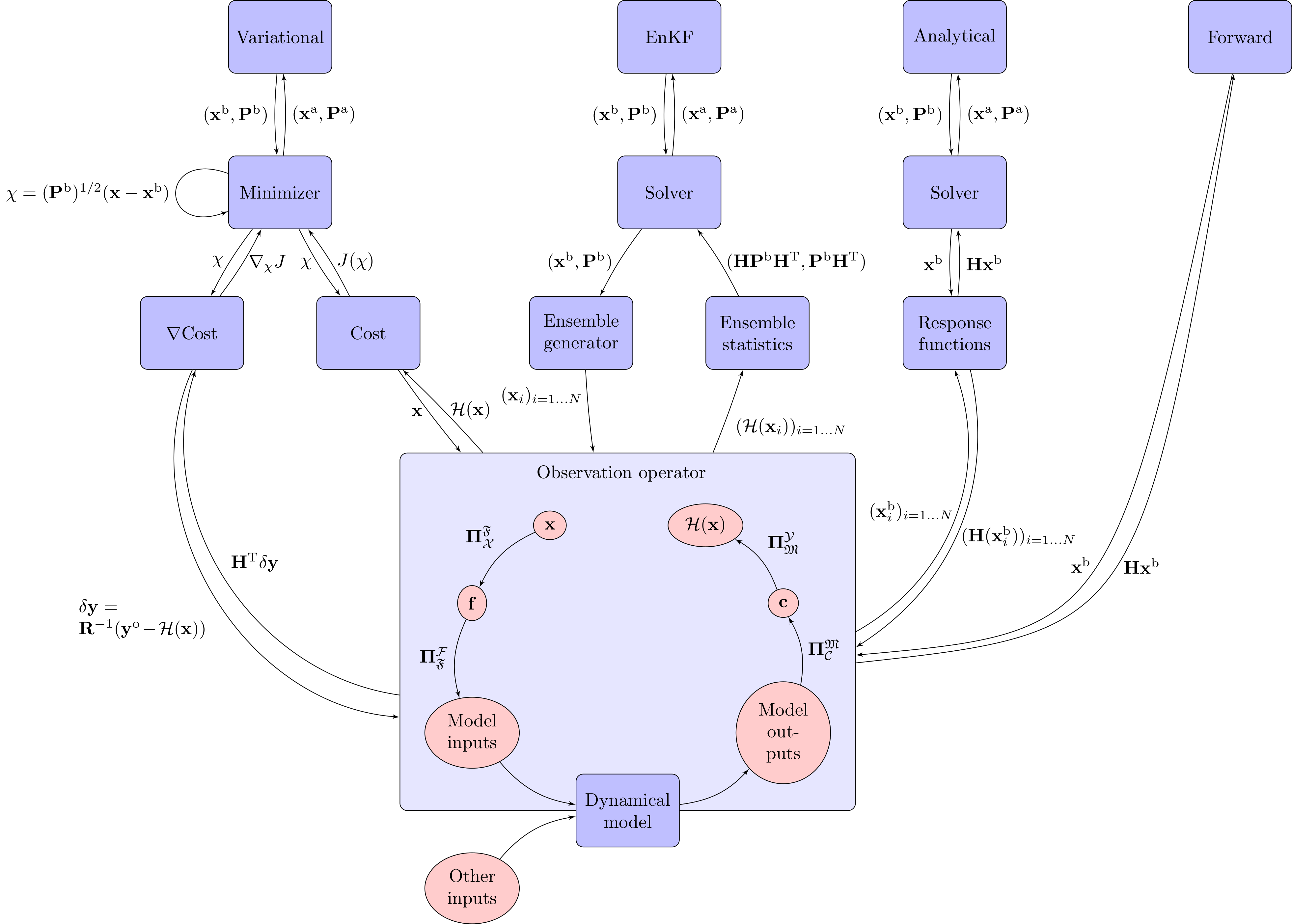
Schematic of the CIF software architecture. Blue boxes indicate plugins explicitly defined in the YAML configuration; red boxes are implicitly loaded from default values. Black arrows represent method dependencies; red arrows represent data dependencies. The observation operator (centre) is the common block shared by all inversion methods.#