Overview

Context

Research institutes have developed various atmospheric inversion systems based on different approaches (regarding e.g. transport model, optimization algorithms, assumption for the inclusion of prior information on the surface fluxes), each having its own strengths and weaknesses. Although referenced in peer-reviewed publications and usually accessible across the research community, these systems are not at the level of transparency, flexibility and accessibility needed to provide the scientific community and policy makers with the most comprehensive and robust view of the uncertainties associated with the inverse estimation of GHG fluxes. Their development, usually carried out by individual research institutes, may in the future not keep pace with the scientific/technical needs to come, such as those to inject the increasing availability of high resolution satellite GHG observations.

The Community Inversion Framework (CIF) is an initiative by members of the atmospheric inversion community to bring together the different approaches, models and inversion systems used in the community. The objective is to benefit from the best of each system, while optimizing dissemination and development efforts.

The CIF is built to run with different atmospheric transport models, regional and global, Eulerian and Lagrangian. This capability will allow errors due to modelled transport to be assessed in a fully consistent framework. A longer-term objective is also to integrate complex schemes needed for FFDAS.

The CIF is designed as a flexible, transparent and open-source tool to estimate the fluxes of different GHGs both at global and regional scales. It combines the best features of existing inversion frameworks and pool efforts for its continued update and revision keeping it state-of-the-art.

Theoretical framework

The CIF should be compatible with analytical inversions, variational inversions, as well as Ensemble Kalman Filters (EnKFs) as the main methods used in the community. All these methods rely on the classical Bayesian inversion framework with Gaussian assumptions. The Gaussian Bayesian formulation of the inversion problem consists in computing the following probability density function (pdf):

(1)\[\begin{equation} p(\mathbf{x} | \mathbf{y}^\textrm{o}, \mathbf{x}^\textrm{b}) \sim \mathcal{N}(\mathbf{x}^\textrm{a}, \mathbf{P}^\textrm{a}) \end{equation}\]

with \(\mathbf{y}^\textrm{o}\) the observation network, \(\mathbf{x}^\textrm{b}\) rendering the prior knowledge on variables to optimize (most of the time fluxes in our case, but also concentration fields in some configurations).

Analytical inversions

When the observation operator is linear, \(\mathcal{H}\) can be fully described by its Jacobian matrix \(\mathbf{H}\), and conversely its adjoint \(\mathcal{H}^*\) by the transpose of the Jacobian \(\mathbf{H}^\textrm{T}\). Thus, \(\mathbf{x}^\textrm{a}\) and \(\mathbf{P}^\textrm{a}\) can be explicitly written as:

(2)\[\begin{split}\begin{equation} \left\{ \begin{array}{rclcl} \mathbf{x}^\textrm{a} & = & \mathbf{x}^\textrm{b} + \mathbf{K}(\mathbf{y}^\textrm{o} - \mathbf{H}\mathbf{x}^\textrm{b}) \\ \mathbf{P}^\textrm{a} & = & \mathbf{P}^\textrm{b} - \mathbf{K}\mathbf{H}\mathbf{P}^\textrm{b} \end{array} \right. \textrm{ or } \left\{ \begin{array}{rclcl} \mathbf{x}^\textrm{a} & = & \mathbf{x}^\textrm{b} + \left[\mathbf{H}^\textrm{T}\mathbf{R}^{-1}\mathbf{H} + (\mathbf{P}^\textrm{b})^{-1}\right]^{-1} \mathbf{H}^\textrm{T}\mathbf{R}^{-1} (\mathbf{y}^\textrm{o} - \mathbf{H}\mathbf{x}^\textrm{b}) \\ \mathbf{P}^\textrm{a} & = & \left[\mathbf{H}^\textrm{T}\mathbf{R}^{-1}\mathbf{H} + (\mathbf{P}^\textrm{b})^{-1}\right]^{-1} \\ \end{array} \right. \end{equation}\end{split}\]

with \(\mathbf{K}\) the Kalman gain matrix: \(\mathbf{K} = \mathbf{P}^\textrm{b}\mathbf{H}^\textrm{T}(\mathbf{R}+\mathbf{H}\mathbf{P}^\textrm{b}\mathbf{H}^\textrm{T})^{-1}\)

The formulation with the Kalman gain matrix is limited by the inversion of a matrix of dimension dim(\(\mathcal{Y}\)), the observation space dimension, while the other formulation is limited by the dimension of the control space. Due to the very high dimensions for both the observation and the control spaces in most inversion applications, the explicit computation of Eq. (2) with matrix products and inverses is not computationally feasible. For this reason, smart adaptations on the inversion framework (including approximations and numerical solvers) are necessary to tackle the problem.

Variational inversions

One possible way to avoid the dimension issue is the variational approach. Computing the normal distribution in Eq. (1) is equivalent to finding the minimum of the cost function:

(3)\[\begin{equation} J(\mathbf{x}) = \frac{1}{2} (\mathbf{x} - \mathbf{x}^\textrm{b})^\textrm{T} (\mathbf{P}^\textrm{b})^{-1} (\mathbf{x} - \mathbf{x}^\textrm{b}) + \frac{1}{2} (\mathcal{H}(\mathbf{x}) - \mathbf{y}^\textrm{o})^\textrm{T} \mathbf{R}^{-1}(\mathcal{H}(\mathbf{x}) - \mathbf{y}^\textrm{o}) \end{equation}\]

In variational inversions, the minimum of the cost function in Eq. (3) is numerically computed using a quasi-Newtonian descending algorithm based on the gradient of the cost function:

(4)\[\begin{equation} \nabla J_\mathbf{x} = (\mathbf{P}^\textrm{b})^{-1} (\mathbf{x} - \mathbf{x}^\textrm{b}) + \mathcal{H}^*\left[\mathbf{R}^{-1}(\mathcal{H}(\mathbf{x}) - \mathbf{y}^\textrm{o})\right] \end{equation}\]

Quasi-Newtonian methods are a group of algorithms designed to compute the minimum of a function. In the community, one example of quasi-Newtonian algorithms commonly used is M1QN3 (Gilbert and Lemaréchal, 1989). In general quasi-Newtonian methods require an initial regularization of \(\mathbf{x}\), the vector to be optimized, for better effileiency. In atmospheric inversion, such a regularization is generally made by optimizing \(\mathbf{\chi} = (\mathbf{P}^\textrm{b})^{-1/2} (\mathbf{x} - \mathbf{x}^\textrm{b})\) instead of \(\mathbf{x}\). Although more optimal regularizations can be chosen, the minimization of the equations with \(\mathbf{\chi}\) is preferred for its simplifying the equation to solve. This transformation translates in Eq. (4) as follows:

(5)\[\begin{equation} \nabla J_\mathbf{\chi} = \chi + (\mathbf{P}^\textrm{b})^{1/2}\mathcal{H}^*\left[\mathbf{R}^{-1}(\mathcal{H}(\mathbf{x}) - \mathbf{y}^\textrm{o})\right] \end{equation}\]

Ensemble Kalman Filters

In EnKFs, such as presented in e.g., Peters et al. (2005), the issue of the high dimension in the system of Equations (2) is avoided using two main procedures:

• observations are assimilated sequentially in the system to reduce the dimension of the observation space, making it possible to compute matrix products and inverses

• covariance matrices are approximated with a Monte Carlo ensemble of possible control vectors:

(6)\[\begin{split}\begin{equation} \label{eq:enkf} \left\{ \begin{array}{rcl} \mathbf{H}\mathbf{P}^\textrm{b}\mathbf{H}^\textrm{T} & \simeq & \frac{1}{N-1}(\mathcal{H}(\mathbf{x}_1), \mathcal{H}(\mathbf{x}_2), ..., \mathcal{H}(\mathbf{x}_N))\cdot(\mathcal{H}(\mathbf{x}_1), \mathcal{H}(\mathbf{x}_2), ..., \mathcal{H}(\mathbf{x}_N))^\textrm{T} \\ \mathbf{P}^\textrm{b}\mathbf{H}^\textrm{T} & \simeq & \frac{1}{N-1}(\mathbf{x}_1, \mathbf{x}_2, ..., \mathbf{x}_N)\cdot(\mathcal{H}(\mathbf{x}_1), \mathcal{H}(\mathbf{x}_2), ..., \mathcal{H}(\mathbf{x}_N))^\textrm{T} \\ \end{array} \right. \end{equation}\end{split}\]

Implementation

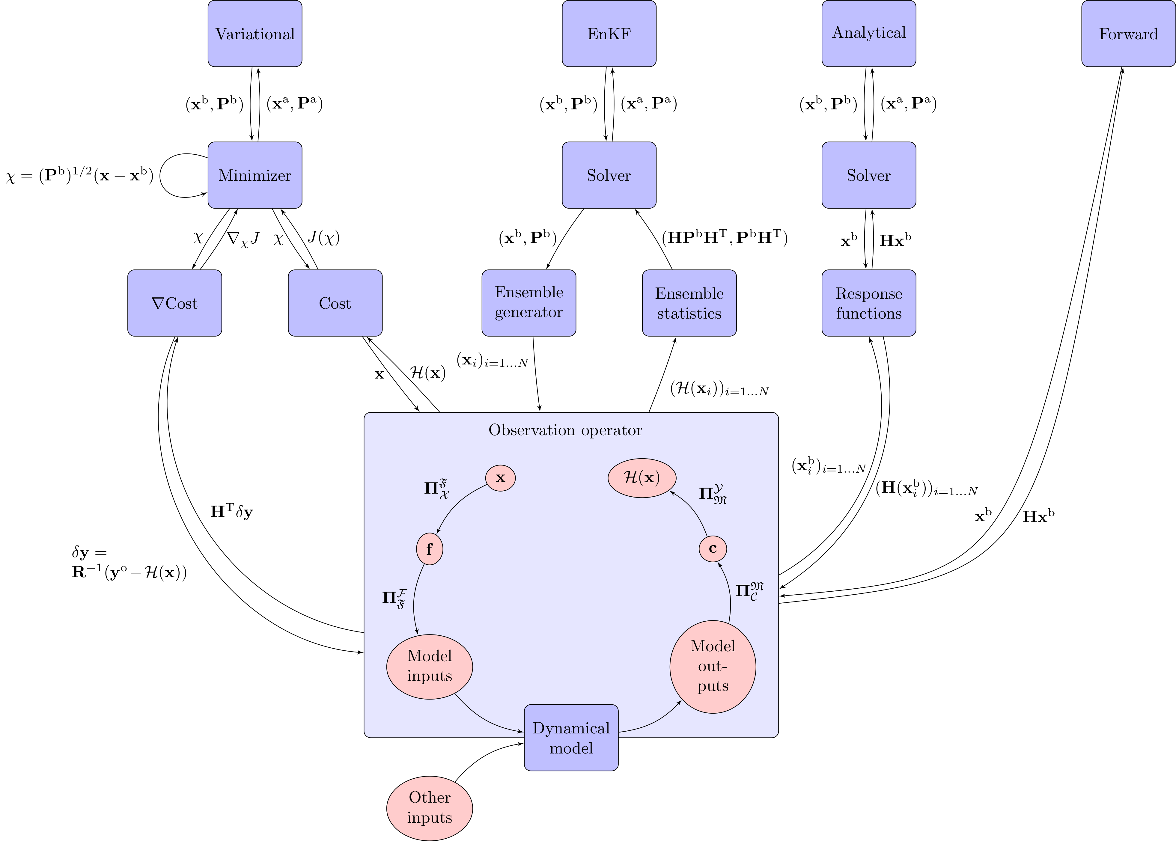
Following Eq. (1) to (6), operating both variational inversions and EnKFs requires the structure summarized below. The generic call graph of the CIF could easily be extended to any other data assimilation method, with the observation operator as the common block between all methods. The observation operator is required to translate information from the control space to the observation space, and reversely in the case of methods using the adjoint. More specific intermediate mappings are required for interfacing the CIF with the chosen dynamical model. They include mappings from/to algebraic spaces used by the inversion to/from practical spaces compatible with the dynamical model inputs and outputs. Such operations depend on the definitions of the control and observation vectors, on the model spatial and temporal resolution, as well as on the format of input and output files for the model.

Please check here for further details on how the CIF blocks are built and linked with each other.